AI - Use Neural Network Model for Training and Prediction (Difficulty: 5)

CreatiCode

Introduction

Neural Network (NN) Models are the core building blocks for many modern AI models, including large language models like ChatGPT.

In this tutorial, you will learn to build a very simple NN model that classifies a random point based on its distance to the origin

Each random point’s x and y coordinates are between -1 and 1. If its distance to the center is less than 0.5, then it will be colored green; otherwise, it will be red. For example, here are 300 random points colored in green or red:

Of course, when we train the model, we will not tell it that the classification is simply based on distance to the origin. Instead, the model has to “figure it out” on its own by analyzing patterns in the training data. Once you know how to train a model, you can solve much more complex problems.

Neurons and Layers

To understand how neural network models work, you need to know what neurons are. A neuron is essentially a weighted sum of its input values.

For example, for a neuron with 2 inputs of x and y, a neuron can be represented by an equation like this:

Suppose the weights w0 and w1 are 0.2 and -0.5, then given any input value of x and y, we can calculate the result value:

x = 0.1 and y = 0.3: result = 0.2 * 0.1 - 0.5 * 0.3 = -0.13
x = 0.8 and y = -0.6: result = 0.2 * 0.8 - 0.5 * (-0.6) = 0.46

Besides these weights, a neuron can also have an activation function, which modifies the result in a certain way.

One popular activation function is called relu: it would set the result to 0 if it is negative. For example, for the case of x = 0.1 and y = 0.3, the initial result is -0.13, then after applying the relu activation, the final result becomes 0.
Another common activation is sigmoid. You can think of it as a “squish” function: it takes any number and turns it into something between 0 and 1. If the number is really big, it comes out close to 1. If it’s small or negative, it comes out close to 0. This is useful when we want the output to act like a probability, as all probability values fall between 0 and 1.

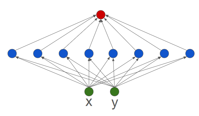
As shown above, a NN model is simply a network of many layers of neurons. Each layer of neurons takes the output of the neurons in the layer below it and applies different weights to them. A neural network can have many layers, and each layer can have many neurons.

Usually the bottom layer is the input layer, and the top layer is the output layer. All other layers between them are called “hidden layers”, since we usally only see the input and output layers of a NN model.

When we build a new NN model, we don’t know the best weights for the neurons, so it is useless. However, through the process of training, the model will gradually figure out the optimal values for these weights.

Now let’s walk through our example step by step.

Step 1 - Starting Project

Please open and remix this project as the starting point:

play.creaticode.com/projects/663058eedc3cd90d25ae3b11

This project contains some basic blocks to add 5 buttons for creating, training, testing, saving and loading NN models. Two empty tables for “training data” and “test data” are also available.

Step 2 - Create an Empty NN Model

When button0 is clicked, we will create an empty NN model like this:

The model will be named “m1”, and we will be using this name to refer to this model in all operations below.

Step 3 - Add a Layer of Neurons

For our model, it needs to guess whether a random point is green or red, so it will take 2 inputs of x and y, which can be thought of as the “bottom layer” or “input layer”. Now, we will add a new layer on top of it. We will choose a layer of 8 neurons like this:

As shown, each of the 8 neurons in the second layer is connected to both inputs, so each neuron will have 2 weight values that need to be trained later.

To add this layer, you can use the “add layer to NN model” block:

A few notes:

Its input shape 2 must match the number of input variables in the first layer (x and y);
Its output size of 8 is the number of neurons in this new layer. If it is too small, the model may not be smart enough; if it is too big, then the model may simply “cheat” by memorizing the training data, and it will fail badly when we test it with new data.
For “activation”, we will choose relu, which will set the calculation result to 0 if it is negative for any neuron. This is a safe option for most situations.

Step 4 - Add the Output Layer

Now let’s add the output layer:

Its input shape must match the output size of the previous layer, which is 8. Since this is the last layer, its output size also has to match the number of variables we are predicting, which is 1. In other words, there is only one neuron in this layer, and it sums up 8 inputs with 8 weights.

The sigmoid activation function is used. As explained earlier, this will convert the weighted sum into a number between 0 and 1.

After this step, we have built a 3-layer model, which takes 2 input variables, calculates 8 values based on them, then aggregate these 8 values into one output variable.

Step 5 - Compile the Model

Now we need to compile the NN model before using it:

This step allows us to configure the model with a few parameters:

The loss calculation method specifies how to calculate errors or mistakes the model is making. For example, in our case, we will give green dots a label of 1, and red dots a label of 0. So if the model’s output for a green dot is very close to 1, then that should be counted as a very samll “loss”. But if the model output is close to 0, then that’s a big “loss”. That is exactly how the “binaryCrossentropy” method works. For other problems, a different way of calculating the loss may be needed.
The optimizer is set to “adam”. This is a commonly used method that controls how the model adjusts its neurons’ weights based on the errors it gets during training. It will look at how the “loss” changes after each training run, and adjust the weights to make the loss smaller.
The learning rate is set to 0.002, which controls how fast we correct the model weights after each training run. If it is a large number, then we make big adjustments to the weights, which might help us find the optimal weights faster for simple cases. However, if the learning rate is too large, we might never find the optimal solution but dancing around it back and forth. Usually, you should pick a learning rate between 0.001 and 0.003.

By now we have completed the model creation, but the model only contains some random weights initially. The next task is to train the model with some data.

Step 6 - Generate Training Data

We will first need to generate some training data. Please define a new block “generate training data”:

Step 7 - Define the “training data” Table

To store the training data, we need to add 3 columns of “x”, “y” and “label” in the “training data” table:

Step 8 - Add Training Data

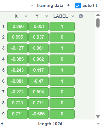
Now we will use a repeat loop to add 1024 rows of data into the “training data” table. For each row, it will have a random number for the x and y values between -1 and 1. Then we will calculate its distance to the origin point. The label will be 1 if the distance is less than 0.5, and 0 otherwise.

Note that this is a simplified example. In practice, there may be more than 2 variables, and the label will also need to reflect the actual classification of each case.

Now if you run the “generate training data” block, you will get 1024 rows of data like this:

Step 9 - Train the NN Model

Now we can use the training data to train the model:

When we “train” the model, this is what happens:

We calculate the output for each input (the pair of x and y values) using the current weights of all neurons in the model.
We calculate the “loss” for each output relative to the given label
We adjust all the weights based on the loss values of a batch of 32 training samples.
We repeat steps 1 to 3 for the next batch.
When all 1024 training samples are processed (a total of 32 batches), we call it a complete epoch. We will start a new epoch with the first batch of samples again.
We will stop after 200 epoches.

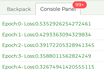
Now, if you click the “Train” button, the training will start, and it will take some time depending on how fast is your computer. During the training, you will see the current loss value printed in the console panel below the editor. The loss value should be descreasing over time, which means the model’s weights are being updated to more accurately predict the labels for all training samples.

For example, at the top of the console panel, you should see the initial “loss” is about -0.53 for epoch 1, and when the training is completed, the loss is reduced to about -0.02:

…

In praictice, suppose you are working on a new problem, and you find the size of the loss staying the same or even incresing, then it means the model is not learning from its mistakes to improve its neurons’ weights. There can be many reasons for why this might happen, and you will need to adjust the model parameters and try again. For example, you can adjust the learning rate, the number and size of the model layers, check the labels of the test data, etc.

Step 10 - Create Test Data

Next, we will test our model to see how well it can predict the label for any new random point. Note that we cannot use any of the training samples for testing, since the model has already “seen” those data, and might have even “memorized” their labels.

When the “test” button is clicked, we will add 4 columns to the test data table. The extra column is prediction, which will be used to store the predicted label from the model.

After that, we will generate 100 rows of data in the test data table using the same method:

When we run this block, we will see some test data with no predictions yet: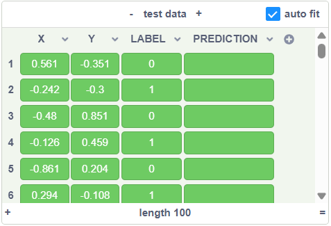

Step 11 - Run the Model for Prediction

Each time the button2 is clicked, we will call the create test data block to generate some new data, and then use the model “m1” to generate prediction for them:

The inputs are:

model name: “m1”
table containing the data: “test data”
rows: we are using row 1 to 100 of this table
input columns: the x and y columns will be used as the 2 input variables for the model
output column: the prediction output will be stored in this column

Here is an example test result:

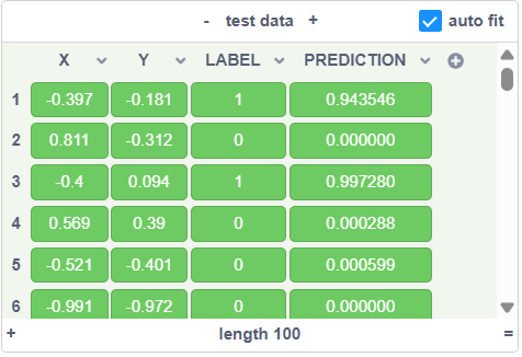
Note that the predictions are very close to the actual labels, but they are still not exactly the same. That’s because the NN model doesn’t really know that the labels are simply the distance to the origin. Instead, it try to guess this relationship by adjusting its neurons repeatedly. However, this is good enough, since its prediction is very close to the label.

Step 12 - Calculate Hit Rate

To measure how well our model did, we can calculate the hit rate using the test data - the percent of times it predicted the label correctly.

Specifically, for each row in the test data, we convert the predicted value to a predicted label: if it is less than 0.5, the predicted label will be 0, otherwise, it will be 1. Then we can count the number of times the predicted label is the same as the actual label.

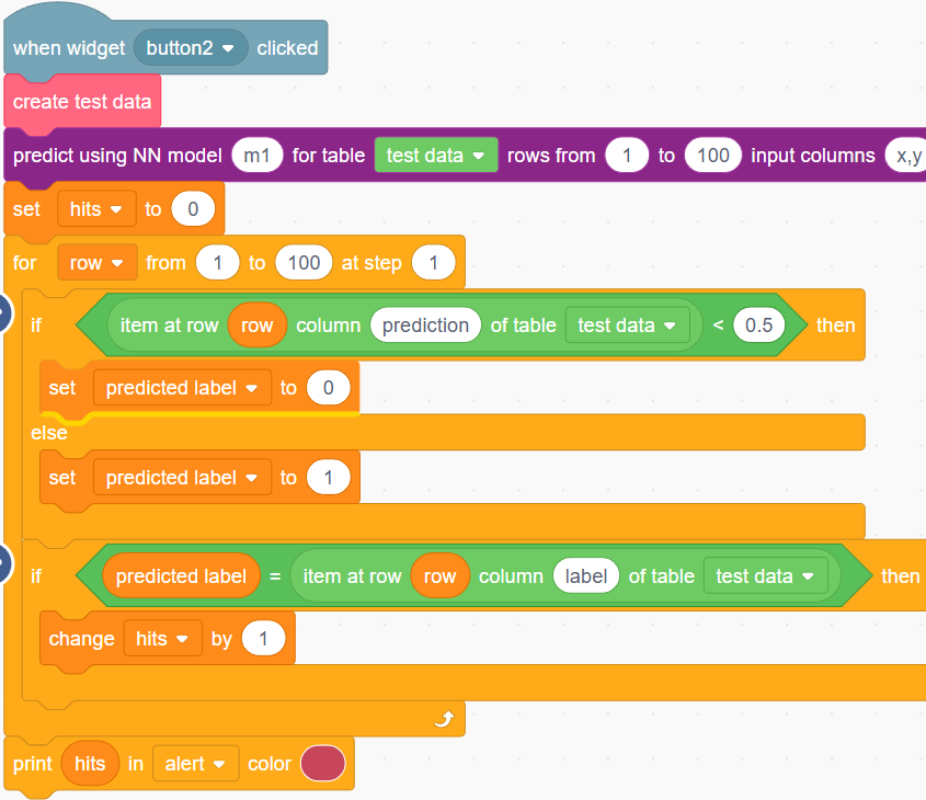
At the end, we are printing out the hit rate, which should be around 97, which is pretty good.

Step 13 - Saving and Loading the Model

If you are building the model for other users, you don’t want to require everyone to train the model. They should be able to simply load the model you have trained and use it for prediction. You can save the model parameters to the CreatiCode server, and then load the model from the server in the future. Note that you can only load models that are saved in the same project.

Here are the blocks:

For a test, try to save the model now, then reload the project. The model will not be available in the playground when you reload the project, so when we test the model, it will not generate any prediction. However, if we load the model, then it can be used to predict again.

Step 14 - Challenges

We have build a model for a relatively simple problem. Here are some new problems you may try next:

Ring Instead of Circle: Classify a random point as 1 when its distance to the origin is between 0.4 and 0.7. If we plot it, it will look like the green area:

Diabetes Dataset: You can reuse the data from this tutorial, with the input variables being “Glucose” and “BMI”, and the label being whether this patient has Diabetes or not. You will need to split the given data into training data and test data.